Digital Comics Data Analysis (Python) - Marvel or DC and some other conclusions
June 06, 2016
The complete code can be found at Github, on the following link: https://github.com/felipegalvao/comixologyscrapingand_analysis
If you prefer, the analysis can also be found in a Jupyter Notebook in https://github.com/felipegalvao/comixologyscrapingand_analysis/blob/master/Comixology%20Analysis%20Notebook%20-%20English.ipynb or https://anaconda.org/felipegalvao/comixology-analysis-notebook-english/notebook
Introduction
After having done the analysis of the Comixology website to prepare for the scraping (post here) and doing the scraping itself to extract the data from the website (post here), we will do a very cool data analysis on the information we extracted, using Python and Pandas.
Let’s find out which publisher has the best prices, the publishers with the best average ratings and a detailed analysis on the giant ones: Marvel x DC Comics. Let’s begin.
Initial Preparation
First, as usual, let’s import the packages we need. They are old friends: numpy, pandas, matplotlib and seaborn. Then, we will read the csv file with the read_csv function from Pandas.
import pandas as pd
import numpy as np
import matplotlib.pyplot as plt
import seaborn as sns

comixology_df = pd.read_csv("comixology_comics_dataset_19.04.2016.csv",
                            encoding = "ISO-8859-1")
Now, let’s create a new column, price per page. This column will help us compare the price of comics that have a different number of pages, and, therefore, should have a bigger price. But how much bigger?
For some comics, the page count information is not available, and so, for these cases, Pandas will return inf as the value of the column, representing an infinite value. For these comics, we will set the price per page as NaN:
# Create price per page column
comixology_df['Price_per_page'] = pd.Series(comixology_df['Original_price'] /
                                            comixology_df['Page Count'],
                                            index=comixology_df.index)

# Define price_per_page as NaN for comics with no information about page count
comixology_df.Price_per_page[comixology_df['Price_per_page'] == np.inf] = np.nan
Now, let’s use the iterrows() function of the DataFrame to extract the publishing year of the print version of the comic. This function creates a for loop that iterates over each row of the DataFrame. Let’s use the split() function to turn the string that contains the print release date into a list of values, and the third one will be the year. In some cases, this will return a value bigger than 2016, and since this is impossible, we will define these cases as NaN:
# Extract the year of release for print version
print_dates = []
for index, row in comixology_df.iterrows():
    if type(comixology_df.ix[index]['Print Release Date']) == float:
        row_year = np.nan
    else:
        row_year = int(comixology_df.ix[index]['Print Release Date'].split()[2])
        if row_year > 2016:
            row_year = np.nan
    print_dates.append(row_year)

comixology_df['Print_Release_Year'] = pd.Series(print_dates,
                                                index=comixology_df.index)
To the analysis (and beyond!)
The first analysis we’ll do is the calculation of some average values of the website, like average price of comics, average page count, among others. We’ll use the nanmean() function from numpy. This function calculates the mean of a series of values, not considering NaN cases.
# Calculate some average values of the site
average_price = np.nanmean(comixology_df['Original_price'])
average_page_count = np.nanmean(comixology_df['Page Count'])
average_rating = np.nanmean(comixology_df['Rating'])
average_rating_quantity = np.nanmean(comixology_df['Ratings_Quantity'])
average_price_per_page = np.nanmean(comixology_df['Price_per_page'])

print("Average Price: " + str(average_price))
print("Average Page Count: " + str(average_page_count))
print("Average Rating: " + str(average_rating))
print("Average Ratings Quantity: " +
      str(average_rating_quantity))
print("Average Price Per Page: " + str(average_price_per_page))

Average Price: 3.69789045383
Average Page Count: 51.5862786864
Average Rating: 4.26347617558
Average Ratings Quantity: 51.5088270335
Average Price Per Page: 0.0805173472536
After that, let’s list comics with an average rating of 5 stars, that have more than 20 ratings (to consider only the more representative comics; comics with an average rating of 5 stars but with only one rating are not a very good metric), and let’s sort it by price per page. In the top, we will have some free comics (the 6 first ones). Then, we will have great comics, in the eyes of the users, that have a very good price.
# List comics with 5 stars rating that have at least 20 ratings
comics_with_5_stars = comixology_df[comixology_df.Rating == 5]
comics_with_5_stars = comics_with_5_stars[comics_with_5_stars.Ratings_Quantity
                                          > 20]
# Print comics sorted by price per page
print(comics_with_5_stars[['Name','Publisher','Price_per_page']].
      sort_values(by='Price_per_page'))

                                                    Name  \
44099                         Left 4 Dead: The Sacrifice
6143                                Looking For Group #1
55253                                The Walking Dead #1
30295  FCBD 2014: Don Rosa's Uncle Scrooge and Donald...
8762                             Mother Russia #1 (of 3)
80022  Scott Pilgrim Vol. 1: Scott Pilgrim's Precious...
50270                 Transformers: The Cover Collection
42749                                  American Elf 2001
42748                                  American Elf 2000
7677                     Cerebus Vol. 2 #2: High Society
                                                 ...
42350                      Elric Vol. 1: The Ruby Throne
70993                           Old Man Logan (2016-) #1
61629      Amazing Spider-Man: Renew Your Vows (2015) #2
65446                           Deadpool (2012-2015) #44
72350                              Spider-Man (2016-) #2
69949  Miles Morales: Ultimate Spider-Man (2014-2015) #6
67030            Giant-Size Little Marvel: AvX (2015) #4
69819                 Master of Kung Fu (2015) #3 (of 4)
72166                       Silver Surfer (2014-2015) #7
74037                    Thanos: The Infinity Relativity

                          Publisher  Price_per_page
44099                         Valve        0.000000
6143                  Blind Ferret         0.000000
55253              Image - Skybound        0.000000
30295                 Fantagraphics        0.000000
8762   Alterna Comics - FUBAR Press        0.000000
80022                     Oni Press        0.000000
50270                           IDW        0.007674
42749         Top Shelf Productions        0.007868
42748         Top Shelf Productions        0.009967
7677              Aardvark-Vanaheim        0.011786
                            ...             ...
42350                         Titan        0.199846
70993                        Marvel        0.207917
61629                        Marvel        0.210000
65446                        Marvel        0.210000
72350                        Marvel        0.210000
69949                        Marvel        0.210000
67030                        Marvel        0.221667
69819                        Marvel        0.221667
72166                        Marvel        0.234706
74037                        Marvel        0.249900
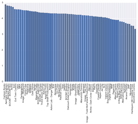
In the next analysis, we will use only comics with more than 5 ratings. For that, we will filter the DataFrame. Then, we’ll create a Pandas pivot table, so that we can visualize the quantity of comics with ratings and the average rating of this publisher. Then, we will consider as representative publishers those that have at least 20 comics with ratings. To do that, we will filter the pivot table. And finally, we will sort this table by average rating, going from the highest to the lowest. This means that the publishers on the top of the table will be the ones that have the best average rating from its comics.
# Filter the original DataFrame for comics with more than 5 ratings
comics_more_than_5_ratings = comixology_df[comixology_df.Ratings_Quantity > 5]

# Create pivot table with average rating by publisher
publishers_avg_rating = pd.pivot_table(comics_more_than_5_ratings,
                                       values=['Rating'],
                                       index=['Publisher'],
                                       aggfunc=[np.mean, np.count_nonzero])

# Filter for any Publisher that has more than 20 comics rated
main_pub_avg_rating = publishers_avg_rating[publishers_avg_rating.
                                            count_nonzero.Rating > 20]
main_pub_avg_rating = main_pub_avg_rating.sort_values(by=('mean','Rating'),
                                                      ascending=False)
print(main_pub_avg_rating)

                                        mean count_nonzero
                                      Rating        Rating
Publisher
Cartoon Books                       4.875000            80
Aardvark-Vanaheim                   4.800000            25
Abstract Studio                     4.786517            89
BOOM! - BOOM! Box                   4.763889            72
Archie                              4.711656           326
Icon                                4.585859           198
Evil Twin Comics                    4.565217            23
Udon                                4.561798            89
MAX                                 4.546911           437
Fantagraphics                       4.518182           110
                                     ...           ...
Asylum Press                        3.898305            59
A Wave Blue World                   3.809524            21
AAM-Markosia                        3.787097           155
Alternative Comics                  3.764706            34
Kickstart                           3.695652            23
Arcana Comics                       3.650794           315
DMP                                 3.636364            99
Moonstone                           3.531915            47
Harlequin/ SB Creative Corp.        3.525641            78
Stormfront Comics                   3.333333            78

[70 rows x 2 columns]
Note that the giants, Marvel and DC Comics, are not among the ones in the top. If we see the complete table, they are between the middle and the bottom of the table.
To help in the visualization, let’s create a matplotlib chart that represents the table above:
# Create chart with average ratings for the Publishers
y_axis = main_pub_avg_rating['mean']['Rating']
x_axis = range(len(y_axis))

plt.bar(x_axis, y_axis)
plt.xticks(x_axis, tuple(main_pub_avg_rating.index),rotation=90)
plt.show()To simplify and have a better table and chart, let’s consider now only the publishers that have 300 comics with ratings. First, the table:
# Filter for Publishers that have more than 300 comics rated
big_pub_avg_rating = publishers_avg_rating[publishers_avg_rating.
                                           count_nonzero.Rating > 300]
big_pub_avg_rating = big_pub_avg_rating.sort_values(by=('mean','Rating'),
                                                    ascending=False)
print(big_pub_avg_rating)

                                        mean count_nonzero
                                      Rating        Rating
Publisher
Archie                              4.711656           326
MAX                                 4.546911           437
Image - Skybound                    4.504092           611
Dark Horse                          4.440000           550
Vertigo                             4.435793          2453
Image                               4.316908          3105
IDW                                 4.313492          2772
Zenescope                           4.309711           381
Oni Press                           4.305376           465
Valiant                             4.291022           323
BOOM! Studios                       4.277219          1194
Avatar                              4.234672           473
DC Comics                           4.218644         13012
Image - Top Cow                     4.176545           793
Image - Todd McFarlane Productions  4.171429           350
Marvel                              4.154245         11177
Dynamite                            4.110597          1944
Arcana Comics                       3.650794           315
And now, the chart that represents the table (less polluted and allowing a better view of the situation of the big publishers):
# Create chart with average ratings for Publishers with more than 300 comics
# rated
y_axis = big_pub_avg_rating['mean']['Rating']
x_axis = np.arange(len(y_axis))

plt.bar(x_axis, y_axis)
plt.xticks(x_axis+0.5, tuple(big_pub_avg_rating.index), rotation=90)
plt.show()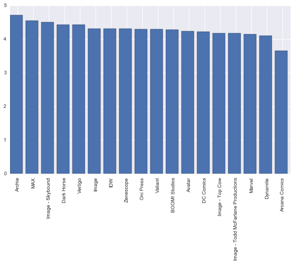
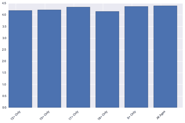
One thing that I believed that could make a difference in the ratings of a comic was the age classification. Were comics made to the adults rated better? Or worse? Let’s check that making another pivot table:
# Create pivot table with Rating by Age Rating
rating_by_age = pd.pivot_table(comics_more_than_5_ratings,
                               values=['Rating'],
                               index=['Age Rating'],
                               aggfunc=[np.mean, np.count_nonzero])

print(rating_by_age)

                mean count_nonzero
              Rating        Rating
Age Rating
12+ Only    4.185380         28304
15+ Only    4.218854          4487
17+ Only    4.341259          9925
18+ Only    4.143939           264
9+ Only     4.360186          1502
All Ages    4.395935          1230
And below, the corresponding chart:
# Bar Chart with rating by age rating
y_axis = rating_by_age['mean']['Rating']
x_axis = np.arange(len(y_axis))

plt.bar(x_axis, y_axis)
plt.xticks(x_axis+0.25, tuple(rating_by_age.index), rotation=45)
plt.show()As we can see, the height of the bars is quite similar. It seems that the age classification does not make a significant effect on the ratings of a comic. If we see it with a purely mathematical view, comics with an age classification for 9+ years or for all ages get the best ratings, by a small margin. But it is not possible to view a strong relation, since it does not varies in the same way as the age classification increases or decreases.
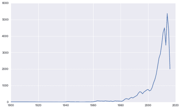
Our next step is to see how the release of comics evolved (considering print versions) over the years. Remember that we already created a column with the year of release of the print version of the comic. The next step is basically to count the occurrences of each year in this column. Let’s make a list with the years and then count the releases per year:
# Create pivot table with print releases per year
print_releases_per_year = pd.pivot_table(comixology_df,
                                         values=['Name'],
                                         index=['Print_Release_Year'],
                                         aggfunc=[np.count_nonzero])
print_years = []
for index, row in print_releases_per_year.iterrows():
    print_year = int(index)
    print_years.append(print_year)
print_releases_per_year.index = print_years
print(print_releases_per_year)

     count_nonzero
              Name
1900            14
1938             1
1939             6
1940             7
1941            21
1942            22
1943            18
1944            13
1945            13
1946            15
           ...
2007          2165
2008          2664
2009          2920
2010          3500
2011          4217
2012          4501
2013          3446
2014          5369
2015          4413
2016          2005

[80 rows x 1 columns]
And now let’s create the cart to see the situation better:
# Create chart with print releases per year
y_axis = print_releases_per_year['count_nonzero']['Name']
x_axis = print_releases_per_year['count_nonzero']['Name'].index
plt.figure(figsize=(10, 6))
plt.plot(x_axis, y_axis)
plt.show()The numbers show that the growing was moderate, until the decade of 2000, when a boom happened, with a great increase in releases until 2012, when the release numbers started to oscillate. The fall shown in 2016 is because we are still in the middle of the year.
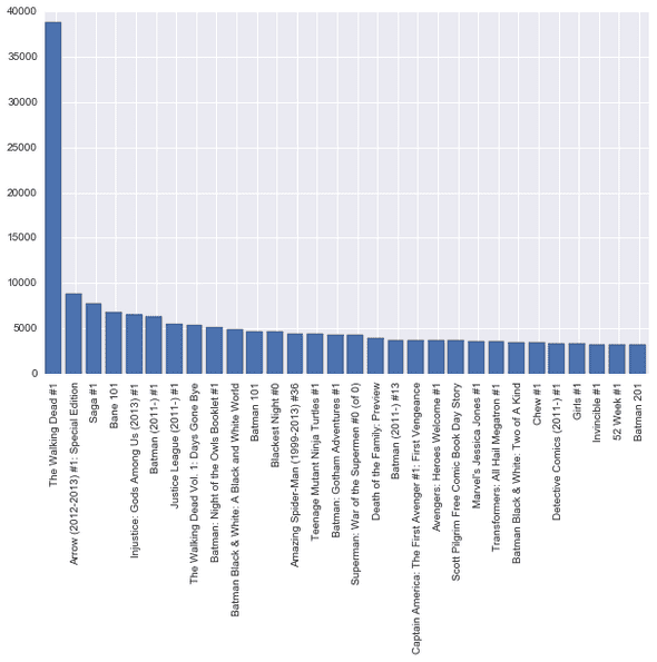
Now we’ll go on to make an evaluation of the most rated comics on the website. We can also probably say that these are the most read comics on the website. So, for this analysis, we will check the comics with most ratings, sorting the table and printing some columns. Let’s see the 30 first ones.
# Sort the DataFrame by ratings quantity and show Name, Publisher and quantity
comics_by_ratings_quantity = comixology_df[['Name','Publisher',
                                            'Ratings_Quantity']].sort_values(
                                            by='Ratings_Quantity',
                                            ascending=False)
print(comics_by_ratings_quantity.head(30))

                                                    Name         Publisher  \
55253                                The Walking Dead #1  Image - Skybound
41479              Arrow (2012-2013) #1: Special Edition         DC Comics
53325                                            Saga #1             Image
11898                                           Bane 101         DC Comics
16638                 Injustice: Gods Among Us (2013) #1         DC Comics
12709                                  Batman (2011-) #1         DC Comics
17286                          Justice League (2011-) #1         DC Comics
55228             The Walking Dead Vol. 1: Days Gone Bye  Image - Skybound
19435               Batman: Night of the Owls Booklet #1         DC Comics
549        Batman Black & White: A Black and White World         DC Comics
231                                           Batman 101         DC Comics
2246                                   Blackest Night #0         DC Comics
61309                 Amazing Spider-Man (1999-2013) #36            Marvel
49490                    Teenage Mutant Ninja Turtles #1               IDW
933                         Batman: Gotham Adventures #1         DC Comics
22805            Superman: War of the Supermen #0 (of 0)         DC Comics
13226                       Death of the Family: Preview         DC Comics
12722                                 Batman (2011-) #13         DC Comics
64194  Captain America: The First Avenger #1: First V...            Marvel
62884                        Avengers: Heroes Welcome #1            Marvel
80024            Scott Pilgrim Free Comic Book Day Story         Oni Press
69771                          Marvel's Jessica Jones #1            Marvel
49753                 Transformers: All Hail Megatron #1               IDW
553                  Batman Black & White: Two of A Kind         DC Comics
51029                                            Chew #1             Image
13749                        Detective Comics (2011-) #1         DC Comics
51699                                           Girls #1             Image
54956                                      Invincible #1  Image - Skybound
40223                                         52 Week #1         DC Comics
232                                           Batman 201         DC Comics

       Ratings_Quantity
55253             38841
41479              8885
53325              7747
11898              6749
16638              6608
12709              6305
17286              5483
55228              5408
19435              5091
549                4920
231                4710
2246               4644
61309              4436
49490              4408
933                4335
22805              4301
13226              3960
12722              3753
64194              3672
62884              3660
80024              3652
69771              3633
49753              3625
553                3489
51029              3434
13749              3303
51699              3279
54956              3275
40223              3248
232                3162
And the chart with the most rated comics:
# Create chart with the previously sorted comics
y_axis = comics_by_ratings_quantity.head(30)['Ratings_Quantity']
x_axis = np.arange(len(y_axis))

plt.bar(x_axis, y_axis)
plt.xticks(x_axis+0.5, tuple(comics_by_ratings_quantity.head(30)['Name']),
           rotation=90)
plt.show()Walking Dead is by far the one with most ratings. After that, some Marvel and DC comics and then some varied ones.
Now, let’s make our detailed analysis on the giant publishers: Marvel and DC Comics.
Marvel vs DC Comics
First, let’s filter the DataFrame, so that only comics from these two remain. After that, we will calculate some average values of these two using a pivot table:
# Filter the DataFrame for comics from Marvel or DC Comics
marvel_dc_comics = comixology_df[(comixology_df.Publisher == 'Marvel') |
                                 (comixology_df.Publisher == 'DC Comics')]

# Create pivot table with Primeiro, alguns valores médios de cada uma
marvel_dc_pivot_averages = pd.pivot_table(marvel_dc_comics,
                               values=['Rating','Original_price','Page Count',
                                       'Price_per_page'],
                               index=['Publisher'],
                               aggfunc=[np.mean])
print(marvel_dc_pivot_averages)

                    mean
          Original_price Page Count Price_per_page    Rating
Publisher
DC Comics       2.600034  35.318463       0.078356  4.233034
Marvel          3.398555  41.344295       0.090946  4.191335
As we can see, DC Comics has a lower average price and price per page, and an average rating slightly higher. The average page count is a little higher on Marvel. Below, the bar charts that represent these comparations:
plt.figure(1,figsize=(10, 6))

plt.subplot(221) # Mean original price
y_axis = marvel_dc_pivot_averages['mean']['Original_price']
x_axis = np.arange(len(marvel_dc_pivot_averages['mean']['Original_price']))
plt.bar(x_axis, y_axis)
plt.xticks(x_axis+0.4,
           tuple(marvel_dc_pivot_averages['mean']['Original_price'].index))
plt.title('Mean Original Price')
plt.tight_layout()

plt.subplot(222) # Mean page count
y_axis = marvel_dc_pivot_averages['mean']['Page Count']
x_axis = np.arange(len(marvel_dc_pivot_averages['mean']['Page Count']))
plt.bar(x_axis, y_axis)
plt.xticks(x_axis+0.4,
           tuple(marvel_dc_pivot_averages['mean']['Page Count'].index))
plt.title('Mean Page Count')
plt.tight_layout()

plt.subplot(223) # Mean Price Per Page
y_axis = marvel_dc_pivot_averages['mean']['Price_per_page']
x_axis = np.arange(len(marvel_dc_pivot_averages['mean']['Price_per_page']))
plt.bar(x_axis, y_axis)
plt.xticks(x_axis+0.4,
           tuple(marvel_dc_pivot_averages['mean']['Price_per_page'].index))
plt.title('Mean Price Per Page')
plt.tight_layout()

plt.subplot(224) # Mean Comic Rating
y_axis = marvel_dc_pivot_averages['mean']['Rating']
x_axis = np.arange(len(marvel_dc_pivot_averages['mean']['Rating']))
plt.bar(x_axis, y_axis)
plt.xticks(x_axis+0.4,
           tuple(marvel_dc_pivot_averages['mean']['Rating'].index))
plt.title('Mean Comic Rating')
plt.tight_layout()

plt.show()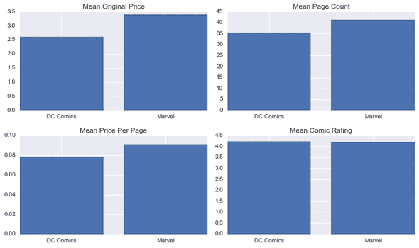
Next step is to see some numbers related to the quantity of comics that each have. How many comics each publisher has, how many of them are good (4 or 5 stars rating), how many are bad (1 or 2 stars) and the proportion of these to the total. For this analysis, we will basically filter the DataFrame and count the number of rows of each filtered view. Simple:
# Calculate total number of comics for each Publisher, proportion of comics
# with rating 4 or bigger and proportion of comics with rating 2 or smaller
marvel_total = len(marvel_dc_comics[marvel_dc_comics['Publisher'] == 'Marvel'])
marvel_4_or_5 = len(marvel_dc_comics[(marvel_dc_comics['Publisher'] == 'Marvel')
                                     & (marvel_dc_comics['Rating'] >= 4)])
marvel_proportion_4_or_5 = marvel_4_or_5 / marvel_total
marvel_1_or_2 = len(marvel_dc_comics[(marvel_dc_comics['Publisher'] == 'Marvel')
                                     & (marvel_dc_comics['Rating'] <= 2)])
marvel_proportion_1_or_2 = marvel_1_or_2 / marvel_total

dc_total = len(marvel_dc_comics[marvel_dc_comics['Publisher'] == 'DC Comics'])
dc_4_or_5 = len(marvel_dc_comics[(marvel_dc_comics['Publisher'] == 'DC Comics')
                                 & (marvel_dc_comics['Rating'] >= 4)])
dc_proportion_4_or_5 = dc_4_or_5 / dc_total
dc_1_or_2 = len(marvel_dc_comics[(marvel_dc_comics['Publisher'] == 'DC Comics')
                                 & (marvel_dc_comics['Rating'] <= 2)])
dc_proportion_1_or_2 = dc_1_or_2 / dc_total

print("\n")
print("Marvel's Total Comics: " + str(marvel_total))
print("Marvel's comics with rating 4 or bigger: " +
      str(marvel_4_or_5))
print("Proportion of Marvel's comics with rating 4 or bigger: " +
      str("{0:.2f}%".format(marvel_proportion_4_or_5 * 100)))
print("Marvel's comics with rating 2 or smaller: " +
      str(marvel_1_or_2))
print("Proportion of Marvel's comics with rating 2 or smaller: " +
      str("{0:.2f}%".format(marvel_proportion_1_or_2 * 100)))
print("\n")
print("DC's Total Comics: " + str(dc_total))
print("DC's comics with rating 4 or bigger: " +
      str(dc_4_or_5))
print("Proportion of DC's comics with rating 4 or bigger: " +
      str("{0:.2f}%".format(dc_proportion_4_or_5 * 100)))
print("DC's comics with rating 2 or smaller: " +
      str(dc_1_or_2))
print("Proportion of DC's comis with rating 2 or smaller: " +
      str("{0:.2f}%".format(dc_proportion_1_or_2 * 100)))
print("\n")

Marvel's Total Comics: 18063
Marvel's comics with rating 4 or bigger: 14791
Proportion of Marvel's comics with rating 4 or bigger: 81.89%
Marvel's comics with rating 2 or smaller: 95
Proportion of Marvel's comics with rating 2 or smaller: 0.53%

DC's Total Comics: 17440
DC's comics with rating 4 or bigger: 15986
Proportion of DC's comics with rating 4 or bigger: 91.66%
DC's comics with rating 2 or smaller: 62
Proportion of DC's comis with rating 2 or smaller: 0.36%
Again, here, DC Comics comes a little better. DC shows a bigger proportion of good comics and a smaller proportion of bad comics. DC scores one more. Below, the chart with the comparisons:
# Create charts with total comics and previously calculated proportions for
# Marvel and DC
plt.figure(2,figsize=(10, 6))

plt.subplot(221) # Total comics for Marvel and DC
y_axis = [dc_total, marvel_total]
x_axis = np.arange(len(y_axis))
plt.bar(x_axis, y_axis)
plt.xticks(x_axis+0.4, ('DC Comics','Marvel'))
plt.title('Total Comics')
plt.tight_layout()

plt.subplot(222) # Proportion of comics with rating 4 or 5
y_axis = [dc_proportion_4_or_5 * 100, marvel_proportion_4_or_5 * 100]
x_axis = np.arange(len(y_axis))
plt.bar(x_axis, y_axis)
plt.xticks(x_axis+0.4, ('DC Comics','Marvel'))
plt.title('Proportion of comics with rating 4 or 5')
plt.tight_layout()

plt.subplot(223) # Proportion of comics with rating 1 or 2
y_axis = [dc_proportion_1_or_2 * 100, marvel_proportion_1_or_2 * 100]
x_axis = np.arange(len(y_axis))
plt.bar(x_axis, y_axis)
plt.xticks(x_axis+0.4, ('DC Comics','Marvel'))
plt.title('Proportion of comics with rating 1 or 2')
plt.tight_layout()

plt.show()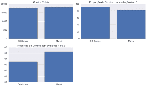
Just as curiosity, let’s check the number of ratings in comics of each publisher, through another pivot table:
# Create Pivot Table with quantity of ratings of each Publisher
marvel_dc_pivot_sums = pd.pivot_table(marvel_dc_comics,
                               values=['Ratings_Quantity'],
                               index=['Publisher'],
                               aggfunc=[np.sum])
print(marvel_dc_pivot_sums)

                       sum
          Ratings_Quantity
Publisher
DC Comics          1725344
Marvel             1099324
Interesting to note that even with Marvel having more comics, as we saw in the previous table, the quantity of ratings of DC’s comics is way bigger, approximately 55% more. It seems that DC’s fans are more propense to rate comics in Comixology than Marvel ones.
Our next evaluation will be about characters and teams of heroes / villains. First, we need to create lists of characters and teams for each publisher. I created the lists by hand, doing some research. It didn’t took very long.
# Define list of characters and teams of DC and Marvel
main_dc_characters = ['Superman','Batman','Aquaman','Wonder Woman', 'Flash',
                      'Robin','Arrow', 'Batgirl', 'Bane', 'Harley Queen',
                      'Poison Ivy', 'Joker','Firestorm','Vixen',
                      'Martian Manhunter','Zod','Penguin','Lex Luthor',
                      'Green Lantern','Supergirl','Atom','Cyborg','Hawkgirl',
                      'Starfire','Jonah Hex','Booster Gold','Black Canary',
                      'Shazam','Catwoman','Nightwing','Zatanna','Hawkman',
                      'Power Girl','Rorschach','Doctor Manhattan',
                      'Blue Beetle','Batwoman','Darkseid','Vandal Savage',
                      "Ra's Al Ghul",'Riddler','Reverse Flash','Black Adam',
                      'Deathstroke','Brainiac','Sinestro','Two-Face']

main_marvel_characters = ['Spider-Man','Captain Marvel','Hulk','Thor',
                          'Iron Man','Luke Cage','Black Widow','Daredevil',
                          'Captain America','Jessica Jones','Ghost Rider',
                          'Spider-Woman','Silver Surfer','Beast','Thing',
                          'Kitty Pride','Doctor Strange','Black Panther',
                          'Invisible Woman','Nick Fury','Storm','Professor X',
                          'Cyclops','Jean Grey','Wolverine','Scarlet Witch',
                          'Gambit','Rogue','X-23','Iceman','She-Hulk',
                          'Iron Fist','Hawkeye','Quicksilver','Vision',
                          'Ant-Man','Cable','Bishop','Colossus','Deadpool',
                          'Human Torch','Mr. Fantastic','Nightcrawler','Nova',
                          'Psylocke','Punisher','Rocket Raccoon','Groot',
                          'Star-Lord','War Machine','Gamora','Drax','Venom',
                          'Carnage','Octopus','Green Goblin','Abomination',
                          'Enchantress','Sentinel','Viper','Lady Deathstrike',
                          'Annihilus','Ultron','Galactus','Kang','Bullseye',
                          'Juggernaut','Sabretooth','Mystique','Kingpin',
                          'Apocalypse','Thanos','Dark Phoenix','Loki',
                          'Red Skull','Magneto','Doctor Doom','Ronan']

dc_teams = ['Justice League','Teen Titans','Justice Society','Lantern Corps',
            'Legion of Super-Heroes','All-Star Squadron','Suicide Squad',
            'Birds of Prey','Gen13', 'The League of Extraordinary Gentlemen',
            'Watchmen']

marvel_teams = ['X-Men','Avengers','Fantastic Four','Asgardian Gods','Skrulls',
                'S.H.I.E.L.D.','Inhumans','A.I.M.','X-Factor','X-Force',
                'Defenders','New Mutants','Brotherhood of Evil Mutants',
                'Thunderbolts', 'Alpha Flight','Guardians of the Galaxy',
                'Nova Corps','Illuminati']
Next, we need to pass each name of character or team. First, let’s define a DataFrame, and we’ll filter so that the only rows that remain are the ones where the comic name includes the name of this character or team. Then, we’ll extract some information from there. The quantity of comics will be the number of rows of the resulting DataFrame. Then, we will get the average price, rating and page count. All this information will be saved in a dictionary, and this dictionary will be appended to a character list, if it is a character, or a team list, if it is a team. In the end, we will have a list of dictionaries for characters and one for teams, and we will use them to create DataFrames:
# Create empty list and dict to hold character info
character_row = {}
characters_dicts = []

for character in main_dc_characters:
    character_df = comixology_df[(comixology_df['Name'].str.contains(character)) &
                                 (comixology_df['Publisher'] == 'DC Comics')]
    character_row['Character_Name'] = character
    character_row['Quantity_of_comics'] = len(character_df)
    character_row['Average_Rating'] = np.nanmean(character_df['Rating'])
    character_row['Average_Price'] = np.nanmean(character_df['Original_price'])
    character_row['Average_Pages'] = np.nanmean(character_df['Page Count'])
    character_row['Publisher'] = "DC Comics"
    characters_dicts.append(character_row)
    character_row = {}

for character in main_marvel_characters:
    character_df = comixology_df[(comixology_df['Name'].str.contains(character)) &
                                 (comixology_df['Publisher'] == 'Marvel')]
    character_row['Character_Name'] = character
    character_row['Quantity_of_comics'] = len(character_df)
    character_row['Average_Rating'] = np.nanmean(character_df['Rating'])
    character_row['Average_Price'] = np.nanmean(character_df['Original_price'])
    character_row['Average_Pages'] = np.nanmean(character_df['Page Count'])
    character_row['Publisher'] = "Marvel"
    characters_dicts.append(character_row)
    character_row = {}

characters_df = pd.DataFrame(characters_dicts)

# Create empty list and dict to hold team info
team_row = {}
teams_dicts = []

for team in dc_teams:
    team_df = comixology_df[(comixology_df['Name'].str.contains(team)) &
                                 (comixology_df['Publisher'] == 'DC Comics')]
    team_row['Team_Name'] = team
    team_row['Quantity_of_comics'] = len(team_df)
    team_row['Average_Rating'] = np.nanmean(team_df['Rating'])
    team_row['Average_Price'] = np.nanmean(team_df['Original_price'])
    team_row['Average_Pages'] = np.nanmean(team_df['Page Count'])
    team_row['Publisher'] = "DC Comics"
    teams_dicts.append(team_row)
    team_row = {}

for team in marvel_teams:
    team_df = comixology_df[(comixology_df['Name'].str.contains(team)) &
                                 (comixology_df['Publisher'] == 'Marvel')]
    team_row['Team_Name'] = team
    team_row['Quantity_of_comics'] = len(team_df)
    team_row['Average_Rating'] = np.nanmean(team_df['Rating'])
    team_row['Average_Price'] = np.nanmean(team_df['Original_price'])
    team_row['Average_Pages'] = np.nanmean(team_df['Page Count'])
    team_row['Publisher'] = "Marvel"
    teams_dicts.append(team_row)
    team_row = {}

teams_df = pd.DataFrame(teams_dicts)
Let’s consider only teams and characters that have more than 20 comics where their names are present on the title of the comic. So, let’s make a filter:
# Filter characters and teams DataFrame for rows where there are more than 20
# comics where the character / team name is present on the title of the comics
characters_df = characters_df[characters_df['Quantity_of_comics'] > 20]
teams_df = teams_df[teams_df['Quantity_of_comics'] > 20]
Now, let’s check the biggest characters and teams in number of comics and average rating. For the characters, even considering the ones with more than 20 comics, there are still too many characters left. So, we’ll limit the list to the top 20 characters. For the teams, there is no need, since there are already less than 20. Then, we’ll print the tables:
# Limit number of characters to 20
top_characters_by_quantity = characters_df.sort_values(by='Quantity_of_comics',
                                         ascending=False)[['Character_Name',
                                         'Average_Rating',
                                         'Quantity_of_comics']].head(20)
top_characters_by_rating = characters_df.sort_values(by='Average_Rating',
                                         ascending=False)[['Character_Name',
                                         'Average_Rating',
                                         'Quantity_of_comics']].head(20)

top_teams_by_quantity = teams_df.sort_values(by='Quantity_of_comics',
                                             ascending=False)[['Team_Name',
                                             'Average_Rating',
                                             'Quantity_of_comics']]
top_teams_by_rating = teams_df.sort_values(by='Average_Rating',
                                           ascending=False)[['Team_Name',
                                           'Average_Rating',
                                           'Quantity_of_comics']]

print(top_characters_by_quantity)

     Character_Name  Average_Rating  Quantity_of_comics
1            Batman        4.218568                2459
47       Spider-Man        4.335099                1680
0          Superman        4.197286                1043
55  Captain America        3.949602                 831
51         Iron Man        4.083821                 744
49             Hulk        4.098540                 707
18    Green Lantern        4.132159                 694
71        Wolverine        4.122517                 631
4             Flash        4.206271                 616
3      Wonder Woman        4.313629                 615
50             Thor        4.251244                 597
54        Daredevil        4.306867                 529
86         Deadpool        4.319018                 504
5             Robin        4.308235                 429
6             Arrow        4.223214                 341
19        Supergirl        4.205036                 296
28         Catwoman        3.920635                 266
2           Aquaman        4.153543                 261
29        Nightwing        4.248869                 221
7           Batgirl        4.307692                 195
Among the characters, we have Batman as the one with the biggest number of comics, followed by Spider-Man and Superman. After that, we have some other famous characters, like Captain America, Iron Man, Wolverine, Flash. Here, nothing surprising.
print(top_characters_by_rating)

        Character_Name  Average_Rating  Quantity_of_comics
115           Mystique        4.666667                  27
25        Booster Gold        4.633803                  83
24           Jonah Hex        4.632911                  84
14   Martian Manhunter        4.611111                  55
35         Blue Beetle        4.542373                  59
59       Silver Surfer        4.468750                  82
64       Black Panther        4.418033                 150
52           Luke Cage        4.388889                  29
83               Cable        4.361111                 144
81              Vision        4.352941                  56
92            Punisher        4.351852                 164
78           Iron Fist        4.348624                 114
96         War Machine        4.347826                  29
69             Cyclops        4.346154                  27
20                Atom        4.336735                 119
47          Spider-Man        4.335099                1680
75                X-23        4.333333                  39
122            Magneto        4.324324                  37
86            Deadpool        4.319018                 504
3         Wonder Woman        4.313629                 615
Here, we have some surprises on the top. Even if the quantity of comics is not very big, few people would imagine that Mystique would be the character with the highest average rating, among all these extremely popular characters. On the next positions, more surprises, with Booster Gold in second, Jonah Hex in third, Blue Beetle in fifth. Of the most popular characters, we see Spider-Man, Deadpool and Wonder Woman, in the end of the top 20. Let’s go to the teams:
print(top_teams_by_quantity)

                  Team_Name  Average_Rating  Quantity_of_comics
11                    X-Men        4.117677                2025
12                 Avengers        4.063710                1721
0            Justice League        4.190608                 744
13           Fantastic Four        4.469671                 632
1               Teen Titans        4.341518                 457
4    Legion of Super-Heroes        4.268966                 326
19                 X-Factor        4.253521                 224
7             Birds of Prey        4.167513                 198
20                  X-Force        4.240838                 193
6             Suicide Squad        4.006329                 159
26  Guardians of the Galaxy        4.132812                 143
3             Lantern Corps        4.125926                 136
22              New Mutants        4.095238                 130
24             Thunderbolts        4.431193                 127
16             S.H.I.E.L.D.        4.053763                 123
21                Defenders        4.066667                  87
2           Justice Society        4.142857                  77
17                 Inhumans        4.245902                  69
10                 Watchmen        4.345455                  55
5         All-Star Squadron        4.500000                  50
8                     Gen13        4.175000                  40
Among the teams with most comics, nothing surprising either. X-Men in first, Avenger in second and Justice League in third. Then, the other teams, like Fantastic Four, Suicide Squad:
print(top_teams_by_rating)

                  Team_Name  Average_Rating  Quantity_of_comics
5         All-Star Squadron        4.500000                  50
13           Fantastic Four        4.469671                 632
24             Thunderbolts        4.431193                 127
10                 Watchmen        4.345455                  55
1               Teen Titans        4.341518                 457
4    Legion of Super-Heroes        4.268966                 326
19                 X-Factor        4.253521                 224
17                 Inhumans        4.245902                  69
20                  X-Force        4.240838                 193
0            Justice League        4.190608                 744
8                     Gen13        4.175000                  40
7             Birds of Prey        4.167513                 198
2           Justice Society        4.142857                  77
26  Guardians of the Galaxy        4.132812                 143
3             Lantern Corps        4.125926                 136
11                    X-Men        4.117677                2025
22              New Mutants        4.095238                 130
21                Defenders        4.066667                  87
12                 Avengers        4.063710                1721
16             S.H.I.E.L.D.        4.053763                 123
6             Suicide Squad        4.006329                 159
On the ratings, the top 3 is formed by the All-Star Squadron, from DC Comics, Fantastic Four and the Thunderbolts, from Marvel. X-Men, Avenger and Suicide Squad are in the end of the list.
Below we plot the charts for these numbers for the characters:
# Create charts related to the characters information
plt.figure(3,figsize=(10, 6))

plt.subplot(121) # Characters by quantity of comics
y_axis = top_characters_by_quantity['Quantity_of_comics']
x_axis = np.arange(len(y_axis))
plt.bar(x_axis, y_axis)
plt.xticks(x_axis+0.4, tuple(top_characters_by_quantity['Character_Name']),
                             rotation=90)
plt.title('Characters by quantity of comics')
plt.tight_layout()

plt.subplot(122) # Characters by average rating
y_axis = top_characters_by_rating['Average_Rating']
x_axis = np.arange(len(y_axis))
plt.bar(x_axis, y_axis)
plt.xticks(x_axis+0.4, tuple(top_characters_by_rating['Character_Name']),
                             rotation=90)
plt.title('Characters by average ratings')
plt.tight_layout()

plt.show()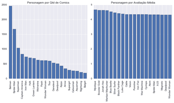
And below, the charts for the teams:
# Creation of charts related to teams
plt.figure(4,figsize=(10, 6))

plt.subplot(121) # Teams by quantity of comics
y_axis = top_teams_by_quantity['Quantity_of_comics']
x_axis = np.arange(len(y_axis))
plt.bar(x_axis, y_axis)
plt.xticks(x_axis+0.4, tuple(top_teams_by_quantity['Team_Name']), rotation=90)
plt.title('Teams by quantity of comics')
plt.tight_layout()

plt.subplot(122) # Teams by average ratings
y_axis = top_teams_by_rating['Average_Rating']
x_axis = np.arange(len(y_axis))
plt.bar(x_axis, y_axis)
plt.xticks(x_axis+0.4, tuple(top_teams_by_rating['Team_Name']), rotation=90)
plt.title('Teams by average ratings')
plt.tight_layout()

plt.show()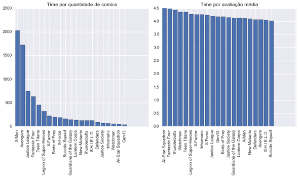
Conclusion
And with that, we conclude our series of 3 posts with the analysis of the website, web scraping and data analysis of digital comics, with information extracted from the Comixology website. As the data is not always available in a simple and practical manner, like a database or a csv dataset, sometimes we have to get the data through web scraping, or some other more complex technique.
In this analysis, we reached some conclusions related to the comics on the website. I made a summary of my conclusions on the list below:
- Some smaller publishers have a good average rating, probably being a good option if you want to read something different than the big ones (Marvel, DC Comics, Image, etc)
- Among the big ones (publishers with more than 300 comics rated on Comixology), Marvel and DC Comics are in the bottom of the ranking when it comes to average ratings of its comics. The three first ones are Archie (of Archie comics, Mega Man, Sonic, among others), MAX (focused in adult comics: Dexter, Jessica Jones, Deadpool) and Image - Skybound (mainly Walking Dead).
- Age Classifications does not seems to affect the rating a comic receives significantly.
- The number of releases of comics increased a lot in the decade of 2000, suffered a recent downfall and now seems to oscilate through the years.
- The two comics with most ratings on Comixology are free. The third, maybe surprisingly, is the first issue of the Saga series, from the publisher Image.
- In the private battle between Marvel and DC Comics, DC seems to have a small advantage. DC has a smaller average price per page and average price, while having a slightly higher average rating. The average page count is a little bigger on Marvel’s comics. DC also has a bigger proportion of good comics (4 ou 5 stars rating) and a smaller proportion of bad comics (1 or 2 stars rating).
- Batman is the character with most comics, followed by Spider-Man and Superman. The heroes with the highest average rating are, surprisingly, Mystique (from X-Men), Booster Gold and Jonah Hex.
- Among the teams, the ones with most comics are the X-Men, Avengers and Justice League. On the podium for the highest average rating are All-Star Squadron from DC, Fantastic Four and Thunderbolts from Marvel.
And with that, we finish our small project. Hope everyone liked. :)
Regards!
